Extracting image data from Whole Slide Images (WSI)

Welcome to SANA (Semi-Automatic Neuropath Analysis)

SANA is a python-based toolkit for processing neuropathology IHC data. In the following examples, we show how SANA can be used to:

1. Read RGB pixel information from WSI’s

2. Extract stain intensity from RGB pixels

3. Classify stain intensity pixels as foreground vs. background

4. Quantify the amount of staining within an image

Part 0: Setup

SANA uses the sana.logging.Logger class to store processing parameters as well as provide information during runtime. Many methods and classes in SANA require this Logger object so we start here.

After, we create a sana.slide.Loader object which prepares us to starting extracting images.

import os
import geojson
import numpy as np
from matplotlib import pyplot as plt

import pdnl_sana.logging
import pdnl_sana.slide
import pdnl_sana as sana

SANAPATH = os.path.expanduser('~/sana_builds/main')

logger = sana.logging.Logger(
    debug_level='full',         # how much information to display to the user
    fpath=f'{SANAPATH}/docs/source/resources/example.pkl'  # stores the processing parameters in a file
)
loader = sana.slide.Loader(
    logger=logger,
    fname=f'{SANAPATH}/docs/source/resources/example.tif', # path to the slide file
    mpp=0.25225                 # microns per pixel resolution constant, often stored in the WSI file
)

# display some information about the slide
print(loader.mpp)
print(loader.ds)
print(loader.level_dimensions)

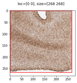
# show the lowest resolution image stored in the WSI
# NOTE: the plotting is done by the logger
thumbnail = loader.load_thumbnail()

0.25225
[ 1.          4.         16.01492537]
((4292, 4292), (1073, 1073), (268, 268))
2025-04-29 13:21:52,517 :: DEBUG :: logging.py :: <func> debug :: Line: 72 :: Loading Frame from .svs slide file...
2025-04-29 13:21:52,537 :: DEBUG :: logging.py :: <func> debug :: Line: 72 :: Done I/O (0.02 sec)

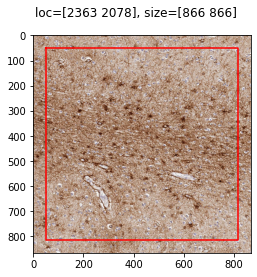
Part 1: Generic ROI

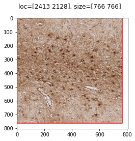
SANA provides a wrapper to the OpenSlide library used to extract RGB images from WSI.

In this example, we provide a set of coordinates which SANA uses to find the bounding box and extracts the relevant information.

# define the ROI within the slide coordinate system
loc = sana.geo.Point(2413, 2128, is_micron=False, level=0)
size = sana.geo.point_like(loc, 766, 766)
roi = sana.geo.rectangle_like(size, loc, size)

# load the sana.image.Frame into memory
frame = loader.load_frame_with_roi(
    roi,
    level=0,
    padding=50,
)

# displaying the parameters used to extract this Frame
print(frame.size())
print(logger.data)

2025-04-29 13:19:24,881 :: DEBUG :: logging.py :: <func> debug :: Line: 72 :: Loading Frame from .svs slide file...
2025-04-29 13:19:25,113 :: DEBUG :: logging.py :: <func> debug :: Line: 72 :: Done I/O (0.23 sec)
[866 866]
{'level': 0, 'angle': None, 'crop_loc': None, 'crop_size': None, 'M': None, 'nw': None, 'nh': None, 'mpp': 0.25225, 'ds': array([ 1.        ,  4.        , 16.01492537]), 'loc': Point([2363, 2078]), 'size': Point([866, 866]), 'padding': 50}

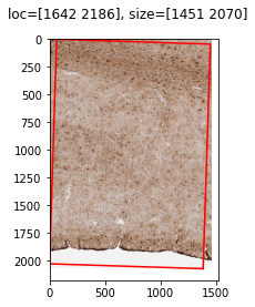
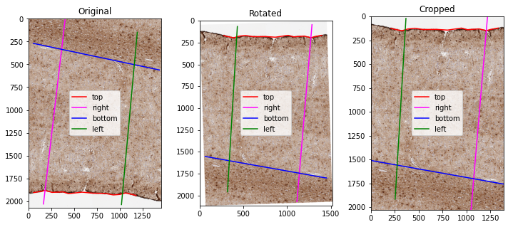
Part 2: Segment-based ROI

An important part of SANA’s capabilities revolve around analyzing a normalized cortical space. In this example, we provide SANA with 4 segments: Top (red), Bottom (blue), Left (green), and Right (pink). This pseudo-quadrilateral is used in future examples to perform a deformation that results in this normalized cortical space. In this example, SANA will use these segments to rotate the source image in order to optimize memory usage

# parses a geojson file containing Polygon or LineString annotations
def load_annotations(f, class_name, roi_name=None):
    out = []
    annotations = geojson.load(open(f, 'r'))["features"]
    for annotation in annotations:
        if annotation["properties"]["classification"]["name"] == class_name and (roi_name is None or annotation["properties"]["name"] == roi_name):
            if annotation["geometry"]["type"] == "Polygon":
                x, y = np.array(annotation["geometry"]["coordinates"][0]).T
                out.append(sana.geo.Polygon(x, y, is_micron=False, level=0))
            elif annotation["geometry"]["type"] == "LineString":
                x, y = np.array(annotation["geometry"]["coordinates"]).T
                out.append(sana.geo.Curve(x, y, is_micron=False, level=0))

    return out

# load the segments
f = f'{SANAPATH}/docs/source/resources/example.geojson'
top = load_annotations(f, "Top", "ROI_0")[0]
right = load_annotations(f, "Right", "ROI_0")[0]
bottom = load_annotations(f, "Bottom", "ROI_0")[0]
left = load_annotations(f, "Left", "ROI_0")[0]

# use the segments to load the data, then rotate and crop the image to minimize memory usage
frame = loader.load_frame_with_segmentations(
    top,
    right,
    bottom,
    left,
    level=0,
    padding=0,
)

# displaying the parameters used to extract this Frame
print(logger.data)

2025-04-29 13:20:03,153 :: DEBUG :: logging.py :: <func> debug :: Line: 72 :: Loading Frame from .svs slide file...
2025-04-29 13:20:03,792 :: DEBUG :: logging.py :: <func> debug :: Line: 72 :: Done I/O (0.64 sec)
{'level': 0, 'angle': 181.82891015687116, 'crop_loc': Point([64.31975168, 43.86412715]), 'crop_size': Point([1386.82052118, 2026.89668716]), 'M': array([[-9.99490584e-01, -3.19150835e-02,  1.51566278e+03],
       [ 3.19150835e-02, -9.99490584e-01,  2.06883432e+03]]), 'nw': 1516, 'nh': 2115, 'mpp': 0.25225, 'ds': array([ 1.        ,  4.        , 16.01492537]), 'loc': Point([1642, 2186]), 'size': Point([1451, 2070]), 'padding': 0}

Part 3: Supplemental ROIs

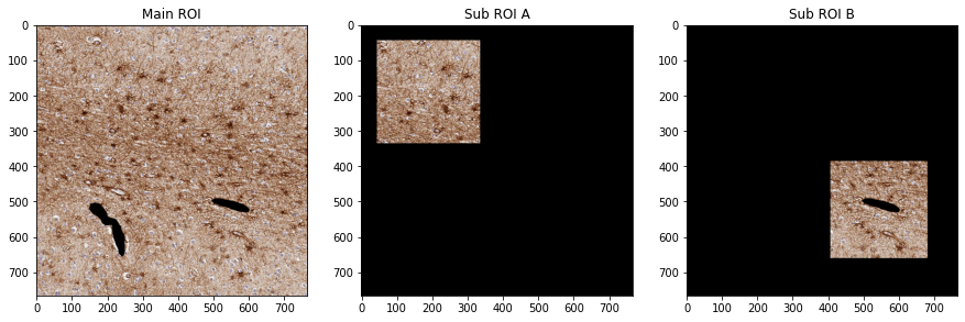
Another major portion of SANA’s capabilities revolves around quantifying processed image masks. In this example, we provide SANA with supplemental ROIs that allow us to generate more quantifiable information. Sub-ROIs (Green/Pink) can be used to calculate data in only specific locations within the Main-ROI (Red). Exclusion-ROIs (Blue) can be used to avoid data within a Main-ROI (Red) entirely

# load the sana.geo.Polygon annotations
f = f'{SANAPATH}/docs/source/resources/example.geojson'
main_roi = load_annotations(f, "ROI")[0]
sub_roi_A = load_annotations(f, "SUB_A")[0]
sub_roi_B = load_annotations(f, "SUB_B")[0]
exclusion_rois = load_annotations(f, "EXCLUDE")

# load the frame data
frame = loader.load_frame_with_roi(roi)

# transform the annotations into the frame's coordinate space
main_roi = sana.geo.transform_array_with_logger(main_roi, logger)
sub_roi_A = sana.geo.transform_array_with_logger(sub_roi_A, logger)
sub_roi_B = sana.geo.transform_array_with_logger(sub_roi_B, logger)
exclusion_rois = [sana.geo.transform_array_with_logger(exclusion_roi, logger) for exclusion_roi in exclusion_rois]

# create the ROI masks based on the annotations
main_mask = sana.image.create_mask_like(frame, [main_roi])
sub_mask_A = sana.image.create_mask_like(frame, [sub_roi_A])
sub_mask_B = sana.image.create_mask_like(frame, [sub_roi_B])
exclusion_mask = sana.image.create_mask_like(frame, exclusion_rois)

# apply the exclusion mask to the ROI masks
main_mask.mask(exclusion_mask, invert=True)
sub_mask_A.mask(exclusion_mask, invert=True)
sub_mask_B.mask(exclusion_mask, invert=True)

# show our work
fig, axs = plt.subplots(1,3, figsize=(15,10))
main_frame = frame.copy(); main_frame.mask(main_mask)
axs[0].imshow(main_frame.img); axs[0].set_title("Main ROI")
sub_frame_A = frame.copy(); sub_frame_A.mask(sub_mask_A)
axs[1].imshow(sub_frame_A.img); axs[1].set_title("Sub ROI A")
sub_frame_B = frame.copy(); sub_frame_B.mask(sub_mask_B)
axs[2].imshow(sub_frame_B.img); axs[2].set_title("Sub ROI B")

2025-04-29 13:20:13,821 :: DEBUG :: logging.py :: <func> debug :: Line: 72 :: Loading Frame from .svs slide file...
2025-04-29 13:20:13,868 :: DEBUG :: logging.py :: <func> debug :: Line: 72 :: Done I/O (0.05 sec)

Text(0.5, 1.0, 'Sub ROI B')

Part 4: Big ROIs (slide scanning)

If an ROI is too big to be loaded into memory, SANA provides a method which creates a grid of smaller Frames which can be loaded/processed separately. Then, the user can aggregate the information during later steps

# load the ROI which defines the tissue within the slide
f = f'{SANAPATH}/docs/source/resources/example.geojson'
tissue_rois = load_annotations(f, 'TISSUE')

# create a grid of 256x256 Frames
# NOTE: we are using level=1 for display purposes, when processing the frames level=0 would likely be required
frame_size = sana.geo.Point(256, 256, is_micron=False, level=1)
framer = sana.slide.Framer(
    loader,
    size=frame_size,
    step=frame_size,
    level=1,
    rois=tissue_rois,
)

# load each frame into memory and plot it
# NOTE: we're
fig, axs = plt.subplots(*framer.nframes, figsize=(15,15))
for i in range(framer.nframes[0]):
    for j in range(framer.nframes[1]):
        frame, mask = framer.load(i, j)
        frame.mask(mask)
        axs[j,i].imshow(frame.img)